Fine-tuning locality-sensitive hashing
Locality-sensitive hashing (LSH) allows for fast retrieval of similar objects from an index - orders of magnitude faster than simple search at the cost of some additional computation and some false positives/negatives. In the last post I introduced LSH for angular distance. In this one I will tell you how you can fine-tune it to get the expected results.
General principle
In general we will fine-tune our system by composing hashing functions belonging to the same group - family. Functions in a family have to meet the following conditions:
- hashes should be more likely to be equal if the items are similar,
- the functions should be statistically independent,
- they should be computationally effective,
- caclculating their composition should be computationally effective.
Now let’s introduce a simple notation:
Let d1 < d2 be the two distances and d a distance function. A family of functions F is (d1, d2, p1, p2)-sensitive if for every f in F and for every item x, y:
- If
d(x, y) ≤ d1, then the probability thatf(x) = f(y)is at leastp1. - If
d(x, y) ≥ d2, then the probability thatf(x) = f(y)is at mostp2
Using this notation we can say that LSH for angular distance from the last post uses a (d1, d2, 1-d1/180, 1-d2/180)-sensitive family of hashing functions.
Composing hashing functions
AND-construction
Given a family of functions F we can compose a new family F' where each f is created by taking r functions from F: {f1, f2, f3, ..., fr}. Then f(x) = f(y) if and only if all of the conditions occur: f1(x) = f1(y), f2(x) = f2(y), … , fr(x) = fr(y).
We did exactly that in the previous post when we started using vectors of dot product signs, as you might remember it lowered chances of two input vectors hashing to the same value.
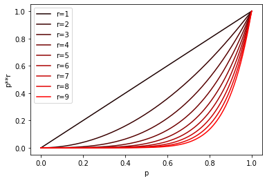
Composing functions in this way lowers all probabilities in our definition. The family F created from (d1, d2, p1, p2)-sensitive family will be (d1, d2, p1**r, p2**r)-sensitive (** - is a Python power operator).
Here’s a chart depicting this transformation for different r values:
OR-construction
We can also compose the a new family using OR semantics. Given a family of functions F we compose a new family F' where each f is created by taking b functions from F: {f1, f2, f3, ..., fb}. Then f(x) = f(y) if and only if at least one of the conditions occurs: f1(x) = f1(y), f2(x) = f2(y), … , fb(x) = fb(y).
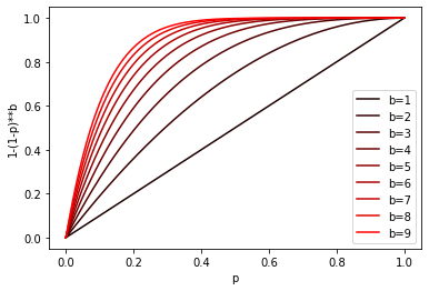
This composition will in turn increase our probabilities. The family F created from (d1, d2, p1, p2)-sensitive family will be (d1, d2, 1 - (1 - p1)**b, 1 - (1 - p2)**b)-sensitive. Here 1 - p is a probability we’ll miss once, (1 - p)**b - is a probability that we’ll miss all the times, so 1 - (1 - p)**b is a probability that we’ll hit at least once.
Here’s chart of the transformation for different b values:
Mixing it together
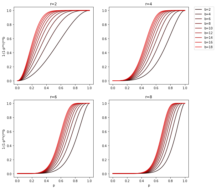
There’s nothing preventing us from applying any of the constructions defined above to a family which is itself a product of a construction. We can for example first use AND construction with r functions from F to get the family F' and then use OR construction with b functions from F' to get the F''. If F was a (d1, d2, p1, p2)-sensitive family, the F'' will be (d1, d2, 1 - (1 - p1**r)**b, 1 - (1 - p2**r)**b)-sensitive.
F'' probability has a sigmoid-like shape, which means that there exists a point (fp) before which probabilities are decreased and after which the probabilities are increased. Thanks to that we can easily manipulate b and r to maximize p1 and minimize p2 for any given d2 < fp < d1 or in other words minimize respectively false-negatives and false-positives. Also steeper the slope, closer the d2 and d1 can be to each other.
It’s easier to grasp this by looking at a chart:
There is of course a drawback to this, stacking AND and then OR construction with r and b functions will require computing r*b hashes. So more functions and/or stacking levels we use, more computation it will require.
Time to code
Let’s now use the knowledge from previous paragraphs and design the index which will put fp at 0.8. The fp can be approximated by (1/b)**(1/r) [1], although it’s not very precise, so you will most likely need to adjust this (sometimes a lot). With the help of:
def s_curve(s, r=1, b=1):
    return 1 - np.power(1 - np.power(s, r), b)
and a chart:
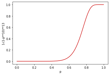
I picked r=10 and b=13, which seem pretty close to what we want: (0.8, 0.771596491730894),(0.81, 0.8145826795188658), (0.8200000000000001, 0.8537120616205055).
Now let’s change the code from previous post to add the OR composition. Each of the vectors will be stored under b keys (a pair of position [0..b-1] and a hash) and when querying we’ll try all b keys against the index.
Also for convenience instead of storing vectors in the dictionary itself we’ll put them in the list and just store their indices. Note than when returning the result we need to make the indices unique as the found candidates could repeat.
Another addition are top_vecs and top_vecs_exact methods which will return n closest vectors to given vector either by using LSH or by comparing to all indexed vectors.
class AngularLSHIndex(object):

    def __init__(self, dim, r, b):
        # dim - dimensionality of used vectors
        # draw b * r random vectors
        self.hash_vecs = np.random.uniform(low=-1.0, size=(b, r, dim))
        # standard python dictionary will be our "index"
        self.db = {}
        self.vecs = []


    def get_hash_key(self, vec):
        # compute dot product of all hash vectors
        # and check the sign
        for i, arr in enumerate(self.hash_vecs):
            sv = vec.dot(arr.T) > 0
            # key is position and bytestring pair
            yield i, np.packbits(sv).tostring()

    def add(self, vec):
        self.vecs.append(vec)
        for k in self.get_hash_key(vec):
            # we store the index of the value under any of the `b` keys
            self.db.setdefault(k, []).append(len(self.vecs)-1)

    def get(self, vec):
        result = set()
        # using set to collect the indices
        # as there might be repeats
        for k in self.get_hash_key(vec):
            if k in self.db:
                result.update(self.db[k])
        return [(idx, self.vecs[idx]) for idx in result]

    def _top_cands(self, vec, cands, n):
        # gets closest vectors in terms of angular_distance
        cand_dist = [(c[0], angular_distance(vec, c[1]), c[1]) for c in cands]
        cand_dist.sort(key=lambda x: x[1])
        if n is not None:
            cand_dist = cand_dist[:n]
        return cand_dist


    def top_vecs(self, vec, n=None):
        # get top vecs by computing distances inside buckets
        cands = self.get(vec)
        return self._top_cands(vec, cands, n)


    def top_vecs_exact(self, vec, n=None):
        # get top vecs by computing all distances
        cands = list(enumerate(self.vecs))
        return self._top_cands(vec, cands, n)
Now let’s try to index some random values and measure the time:
VEC_NO = 10000
VEC_DIM = 10
r = 10
b = 13

vec_set = np.random.uniform(low=-1.0, size=(VEC_NO, VEC_DIM))
idx = AngularLSHIndex(VEC_DIM, r, b)

t0 = time.time()

for vec in vec_set:
    idx.add(vec)

print(time.time() - t0)
#>>> 0.628241777420044
Let’s imagine that our index will be used to get 5 closest vectors to any given vector. Let’s test how our index will fare in this task. First we’ll generate some random vectors:
TEST_SIZE = 100
test_set =  np.random.uniform(low=-1.0, size=(TEST_SIZE, VEC_DIM))
Now we’ll use our index:
TOP_N = 5
t0 = time.time()
approx_results = []
for vec in test_set:
    approx_results.append(idx.top_vecs(vec, TOP_n))
print(time.time() - t0)
# 0.559455156326294
t0 = time.time()
exact_results = []
for vec in test_set:
    exact_results.append(idx.top_vecs_exact(vec, TOP_N))
print(time.time() - t0)
# 9.336578130722046
We can now compute precision and recall:
tp, fp, fn = 0, 0, 0
for a_res, e_res in zip(approx_results, exact_results):
    a_s = set([d[0] for d in a_res])
    e_s = set([d[0] for d in e_res])
    tp += len(a_s.intersection(e_s))
    fp += len(a_s.difference(e_s))
    fn += len(e_s.difference(a_s))
print('Precision: {}, Recall: {}'.format(tp / (tp + fp), tp / (tp + fn)))
# Precision: 0.932, Recall: 0.932
The precision and recall are not perfect but the LSH approach is over 16 times faster. For the full picture here’s a histogram of all distances returned by the top_vecs_exact method:
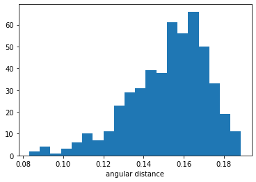
As you can see most values are not very close to query vector, which should explain why precision and recall are not higher for this data.
The end
Thanks for the reading. The LSH is a great technique, which can speed up many tasks, but at the cost of precision and recall. I hope after reading this post you will be able to fine-tune it according to your needs. Stay tuned for more posts about the LSH.